In the first article on linear regression I promised to show how to do it better, so this post will be about truly scientific approach to the problem. Don’t worry if you don’t get it off hand. Honestly speaking it took some time for me to figure out what’s going on and even now from time to time I take some paper and draw matrices/vectors to be sure I’m doing everything right.

First let’s consider fairly simple example. Suppose you were given following column vector: $$ \vec{X} = \begin{bmatrix} x_1 \\\
x_2 \\\
\vdots \\\
x_n \end{bmatrix} $$

and you need to find sum of $ x_{n}^{2} $. I understand that it’s trivial and synthetic example, but later all these over-complications will come handy.

First that that came in mind is just to make iteration over $ x_n $ and accumulate values like below.

print sum([x**2 for x in range(1, 5)])

but that’s too easy and not cool at all. We’re going to use the power of linear algebra here. Fortunately I took linear algebra class in the university and it’s good time to resurrect the knowledge and give it a chance. Matrix multiplication works well here.

So to get sum of squared vector elements we will use following formula $$ \text{sum} = \begin{bmatrix} x_1 & x_2 & \cdots & x_n \end{bmatrix} * \begin{bmatrix} x_1 \\\
x_2 \\\
\vdots \\\
x_n \end{bmatrix} = \vec{X}^T * \vec{X} $$

Now let’s look at our problem from the first post. We have pairs of $ (x^{(i)}, y^{(i)}) $ and hypothesis $ y = \theta_0 + \theta_1*x $ . If we look at this task from the slightly different angle we will see that we were given two column vectors. One for $ X $ values as input and second for $ Y $ values as our output. Let’s rewrite our hypothesis in following form to make it even more obvious $ y = \theta_0*1 + \theta_1*x $. Clear now? If not, don’t worry, below I’ll give detailed explanation of all the steps.

It’s easy to see (frankly saying it was not so obvious until I was told about it) that formula for $ Y $ looks as matrix multiplication, where $ \theta $ is column vector $$ \theta = \begin{bmatrix} \theta_0 \\\ \theta_1 \end{bmatrix} $$ and $ X $ is $ m\times 2 $ matrix, where m is the size of our dataset. So let’s rewrite it as

$$ h_{\theta}(x) = \begin{bmatrix} 1 & x_1^{(1)} \\\
1 & x_1^{(2)} \\\
\vdots & \vdots \\\
1 & x_1^{(m)} \end{bmatrix} * \begin{bmatrix} \theta_0 \\\
\theta_1 \end{bmatrix} = \begin{bmatrix} y^{(1)} \\\
y^{(2)} \\\
\vdots \\\
y^{(m)} \end{bmatrix} $$ And let’s call all those ones as $ x_0^{(i)} $ So cost function can be rewritten in the the following vectorized form $$ J(\theta) = \frac{1}{2m}\sum_{i=0}^{n} (h_\theta(x^{(i)}) - y^{(i)})^2 = \frac{1}{2m}\text{sum}((X*\theta - Y)^2) $$

Code for partial derivatives of $ J(\theta) $ function can be also vectorized. It was a brain teaser to write all $ \theta_j $ update in one step but when it’s done it seems really obvious.

We have vectorized form of $ h_{\theta}(X) - Y $ and to calculate all partial derivatives that are now written in form $$ \frac{\partial}{\partial \theta_j} J(\theta_j) = \frac{1}{m}\sum_{i=0}^{n} (h_\theta(x^{(i)}) - y^{(i)})x_{j}^{(i)} $$ since $ x_{0}^{(i)} = 1 $ Our $ \theta $ is a column vector so to decrease it we have to have the same column vector for its gradient.

Dimension of $ h_{\theta}(X) - Y $ is $ m\times 1 $ and dimensions of $ X $ with $ x_0 $ column added is $ m\times 2 $, so to get $ \sum_{i=0}^{n} (h_\theta(x^{(i)}) - y^{(i)})x_{j}^{(i)} $ we can transpose our $ X $ matrix to $ 2\times m $ one and multiply it with the $ h_{\theta}(X) - Y $ subtraction resulting vector. Below is the full formula for gradient descent $$ \vec{\theta} = \vec{\theta} - \frac{\alpha}{m}X^T*(h_\theta(X) - Y) $$

And that’s really it. We have our function parameters updated in one step. There are lots of advantages of the vectorized implementation. You don’t need to bother with all those for loops when you have $ X $ with multiple features (here we have just one, but in next posts we will deal with multiple features and polynomial regression). Second as all calculations are rarely done by hand, more often by some libraries such as numpy in python, they will be faster because all libraries are highly optimized and use operations parallelism, thus vectorized approach will run much faster.

And below is the code for the vectorized implementation.

import matplotlib.pyplot as plt
import numpy as np

def costFunction(theta, x, y):
    return (sum((x.dot(theta) - y) ** 2) / (2 * x.shape[0]))[0]

def gradientDescent(theta, x, y):
    m = y.size;
    numiter = 1500
    alpha = 0.01
    costHistory = []
    for i in range(0, numiter):
        theta = theta - (alpha / m) * np.transpose(x).dot(x.dot(theta) - y)
        costHistory.append(costFunction(theta, x, y))
    return costHistory, theta

data = np.loadtxt('ex1data1.txt', delimiter=',')

X = data[:, 0]
Y = data[:, 1]
Y = Y.reshape((Y.size, 1))
m = X.size

t = np.ones(shape=(m, 2))
t[:, 1] = X
X = t;
theta = np.array([0, 0])
theta = theta.reshape((2, 1))

costHistory, theta = gradientDescent(theta, X, Y)

plt.xlabel("Iterations count")
plt.ylabel("J($\\theta$) value")
plt.axis([0, 1500, min(costHistory), max(costHistory)])

plt.plot(range(0, 1500), costHistory)

plt.show()

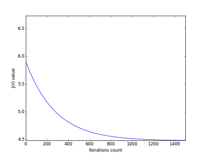
Since function the same as in the first post, I won’t show it here. Instead let’s look at gradient work. We will see how cost function $ J(\theta) $ is getting lower and lower with each step of gradient descent.