I’m taking cool Machine Learning class at Coursera, so to get better understanding of the material, decided to write a series of blog posts about it. As it clear from the post title, I’m going to explain what linear regression is and how it works. I don’t like to read long-long posts because somewhere in the middle I can’t get rid of feeling that the beginning of the post became vague and most of facts were forgotten. So it’s going to be short and painless.

Linear regression

Linear regression is the way to model relationship between input variables $ X $ and output values $ Y $ using linear function. Our model fits in form $$Y = \theta_0 + \theta_1*X_1 + … +\theta_n*X_n$$ where $ \theta_n’s $ are coefficients for linear function above. So when function is found it’s possible to predict $ Y $ value for new $ X $ that does not fall in range of known inputs.

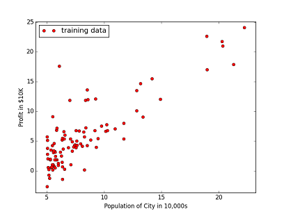
Suppose you have several stores across the country and going to open couple new ones. You need to estimate how profitable will it be if it’s opened in one city or another. The data describing profit of existing stores are presented below as a bunch of points at the scatter plot

Now linear parameter must be chosen to draw a straight line lying as close to each point as possible. In other words our goal is to minimize cost function $ J(\theta) $: $$ J(\theta) = \frac{1}{2m}\sum_{i=0}^{n} (h_\theta(x^{(i)}) - y^{(i)})^2 $$ where $ h_\theta(x) $ is our linear function and paramters are $ \theta $ values.

To find the mininum (global or local, it depends on function) of the function we will use gradient descent method. It is based on on fact that differentiable function decreases in the gradient direction. So basic formula to adjust $ \theta $ parameters using batch gradient descend is: $$ \theta_j = \theta_j - \alpha \frac{\partial}{\partial \theta_j} J(\theta_j) $$ If you have taken calculus course it is easy to calculate partial derivative by hand, but don’t worry if you didn’t get it. Below is calculated derivatives and formula for the $ \theta_i $ update. $$ \frac{\partial}{\partial \theta_j} J(\theta_j) = \frac{1}{m}\sum_{i=0}^{n} (h_\theta(x^{(i)}) - y^{(i)}) \space \text{if j = 0} $$

it is for the first coefficient $ \theta_0 $

$$ \frac{\partial}{\partial \theta_j} J(\theta_j) = \frac{1}{m}\sum_{i=0}^{n} (h_\theta(x^{(i)}) - y^{(i)})x_{j}^{(i)} \space \text{if j > 0} $$

Important point: all $ \theta $ values should be updated simultaneously, i.e. we calculate all new thethas using the old ones first, store them in temporary variables and then at the end of iteration update all theta values.

With each gradient descent step our $ \theta $ values will be closer to the optimal values and cost function $ J(\theta) $ will be closer to its minimum.

Full code of the naive implementation is below.

import numpy as np
import matplotlib.pyplot as plt


def costFunction(theta, x, y):
    cost = 0
    for i in zip(x, y):
        cost = cost + ((h(theta, i[0]) - i[1]) ** 2);
    return cost / (2 * len(x))

def h(theta, x):
    return theta[0] + theta[1] * x

def gradientDescent(x, y):
    # initialize alpha value
    alpha = 0.01
    iternum = 1500
    # set up initial theta values
    theta = [0, 0]
    for i in range(0, iternum):
        theta_0 = 0
        theta_1 = 0
        for i in zip(x, y):
            theta_0 += (h(theta, i[0]) - i[1])
            theta_1 += (h(theta, i[0]) - i[1]) * i[0]

        theta[0] = theta[0] - alpha*theta_0 / len(x)
        theta[1] = theta[1] - alpha*theta_1 / len(x)

    return theta;

f = open('ex1data1.txt')
a = zip(*[[float(l.split(',')[0]), float(l.split(',')[1])] for l in f.readlines()])

x = a[0]
y = a[1];
minX = min(*x)
maxX = max(*x)
minY = min(*y)
maxY = max(*y)

plt.xlabel("Population of City in 10,000s")
plt.ylabel("Profit in $10K")
plt.axis([min(*x) - 1, max(*x) + 1, min(*y) - 1, max(*y) + 1])

plt.plot(x, y, 'ro', label='training data')

tt = gradientDescent(x, y)
print(tt)
xn = np.arange(minX, maxX, 1)
plt.plot(xn, tt[0] + tt[1]*xn, label='Linear function')


plt.legend(loc=2)
plt.show()

Final rounded theta values calculated by the code are $ \theta_0 = -3.6302 $ and $ \theta_1 = 1.1664 $

And our linear function with minimal distance to the training data set is shown at the plot below.

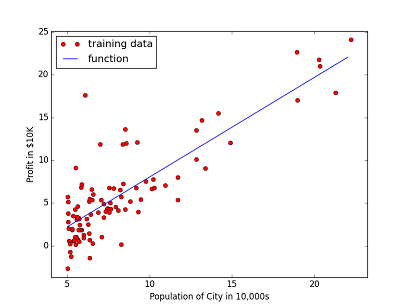
Now using our theta values we can estimate profit for a city with 50K citizens. It is approximately 547.000 $

In my next post I’m going to explain how to choose $ \alpha $ values, and how to implement it better (certainly it can be done better). It’s on the way.